Example 3LC1. Linear model: US production function (48 states in 9 regions)

Baltagi, Song and Jung (2001) estimated a Cobb Douglas production function for the US productivity data of Munnell (1990) for the period 1970-1986. The data set (productivity.dat) contains information by year, state and region on various capital and labour inputs. The same data were used by Rabe-Hesketh and Skrondal (2005, exercise 7.3). The data are for 48 US states (level 2) and 9 regions of the US (level 3). We estimate a 3-level model of the logarithm of private capital stock, using some of the state-level measures of unemployment and various publicly funded activities as covariates.

References

Baltagi, B. H., S. H. Song, and B. C. Jung, (2001), Journal of Econometrics 101: 357–381.

Munnell, A., (1990), Why has productivity growth declined? Productivity and public investment. New England Economic Review. Jan. / Feb.:3–22.

Rabe-Hesketh, S., and Skrondal, A., (2005), Multilevel and Longitudinal Modelling using Stata, Stata Press, Stata Corp, College Station, Texas.

Data description

Number of observations = 816

Number of level 2 cases (‘state’ = states of U.S.) = 48

Number of level 3 cases (‘region’ = region of U.S.) = 9

Number of variables (columns): 17

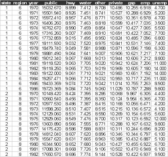
The variables are:

state = states 1-48

region = regions 1-9

year = years 1970-1986

public = public capital stock

hwy = log(highway component of public capital stock)

water = log(water component of public capital stock)

other = log(bldg/other component of public capital stock)

private = log(private capital stock)

gsp = log(gross state product)

emp = log(non-agriculture payrolls)

unemp = state unemployment rate

The first few lines of productivity.dat look like:

Example

We will start by estimating a linear model (without random effects) for the logarithm of private capital stock, private with the covariates hwy, water, other and unemp.

We will then allow for both the state random effect (state) and for the region random effect (region), using mass 96 for both level 2 and level 3.

Both these random effects are significant and significant, sclev2= 0.29718 (0.46362E-02), sclev3=0.25728 (0.59759E-02), and sclev2> sclev3.

Sabre commands

out productivity.log

data state region year public hwy water other private gsp emp unemp

read productivity.dat

case first=state second=region

yvar private

family g

constant cons

mass first=96 second=96

alpha 1

ari a

fit hwy water other unemp cons

dis m

dis e

stop

Sabre log file

<S> data state region year public hwy water other private gsp emp unemp

<S> read productivity.dat

816 observations in dataset

<S> case first=state second=region

<S> yvar private

<S> family g

<S> constant cons

<S> mass first=96 second=96

<S> alpha 1

<S> ari a

<S> fit hwy water other unemp cons

Initial Homogeneous Fit:

Iteration Log. lik. Difference

__________________________________________

1 -92.779046

Iteration Log. lik. Step End-points Orthogonality

length 0 1 criterion

________________________________________________________________________

1 103.83069 1.0000 fixed fixed 10.740

2 164.91413 1.0000 fixed fixed orthogonal

3 223.61434 1.0000 fixed fixed 42.534

4 398.66698 0.2500 fixed fixed 31.955

5 566.38688 1.0000 fixed fixed 115.99

6 570.93147 0.5000 fixed fixed 246.80

7 620.84031 1.0000 fixed fixed 4.2063

8 623.61855 0.0313 fixed fixed 2.0443

9 644.67990 0.0625 fixed fixed 1.0336

10 650.52590 0.0156 fixed fixed 6.8368

11 656.76716 0.2500 fixed fixed 190.53

12 818.89009 1.0000 fixed fixed orthogonal

13 819.90069 1.0000 fixed fixed 30.958

14 821.07209 0.5000 fixed fixed 16.374

15 821.12792 0.0156 fixed fixed 4.1429

16 821.43748 0.0313 fixed fixed orthogonal

17 823.01496 1.0000 fixed fixed orthogonal

18 824.22349 1.0000 fixed fixed orthogonal

19 825.35265 1.0000 fixed fixed orthogonal

20 826.26399 1.0000 fixed fixed orthogonal

21 827.09599 1.0000 fixed fixed 11.708

22 827.21836 0.0078 fixed fixed orthogonal

23 827.86688 1.0000 fixed fixed 1.9105

24 827.88532 0.0020 fixed fixed 5.2971

25 828.22338 0.0313 fixed fixed orthogonal

26 830.19284 1.0000 fixed fixed 13.645

27 830.88480 0.5000 fixed fixed 21.926

28 831.07719 0.0625 fixed fixed orthogonal

29 833.75857 1.0000 fixed fixed 6.6293

30 837.85297 0.1250 fixed fixed 14.817

31 838.95540 0.0313 fixed fixed 1.7552

32 839.49882 0.0313 fixed fixed 23.321

33 839.69707 0.0625 fixed fixed 541.01

34 845.39686 1.0000 fixed fixed orthogonal

35 845.68906 1.0000 fixed fixed 47.137

36 845.75796 1.0000 fixed fixed 1.8814

37 847.99216 0.0156 fixed fixed 83.612

38 849.76283 0.1250 fixed fixed orthogonal

39 850.45014 1.0000 fixed fixed 21.772

40 851.83832 0.0625 fixed fixed 102.61

41 852.42080 0.0625 fixed fixed 3.2700

42 852.50899 0.0078 fixed fixed 67.357

43 854.46818 0.1250 fixed fixed 7242.5

44 855.63389 1.0000 fixed fixed 1092.9

45 856.11039 0.0625 fixed fixed 20.617

46 856.21877 0.0039 fixed fixed 12.124

47 856.25543 0.0039 fixed fixed 6.6368

48 857.06500 0.0020 fixed fixed 21.259

49 857.35161 0.0078 fixed fixed 992.65

50 857.61633 1.0000 fixed fixed 2620.9

51 859.23405 0.5000 fixed fixed 1816.3

52 859.84857 1.0000 fixed fixed 3010.6

53 859.92138 1.0000 fixed fixed 11616.

54 859.92154 1.0000 fixed fixed 2188.8

55 859.92154 1.0000 fixed fixed

<S> dis m

X-vars Y-var Case-var

________________________________________________

cons private state

hwy region

water

other

unemp

Univariate model

Standard linear

Gaussian random effects

Number of observations = 816

Number of level 2 cases = 48

Number of level 3 cases = 9

X-var df = 5

Sigma df = 1

Scale df = 2

Log likelihood = 859.92154 on 808 residual degrees of freedom

<S> dis e

Parameter Estimate Std. Err.

___________________________________________________

cons 1.5157 0.53379E-01

hwy 0.35939 0.13771E-01

water 0.56907 0.12396E-01

other 0.18537 0.13000E-01

unemp 0.21874E-02 0.13306E-02

sigma 0.71069E-01 0.17798E-02

sclev2 0.29718 0.46362E-02

sclev3 0.25728 0.59759E-02

<S> stop