Example
3LC2. Binary response model: Guatemalan mothers using prenatal care for their
children (1558 mothers in 161 communities)
The data (guatemala_prenat.dat) we use in this example are from Rodríguez and Goldman (2001), and are about the use of modern prenatal care. The data set has 2449 observations on children with a binary indicator for whether the mother had prenatal care, there are 25 covariates. The variables include the level-2 mother identifier (mom), the community or cluster (level-3) identifier, a binary indicator of the use of prenatal care for each child and other child-family, and community-level explanatory variables. The explanatory variables are either continuous variables (pcind81: proportion indigenous in 1981 and ssdist: distance to nearest clinic) or 0-1 dummy variables (all others) representing discrete factors coded using the reference categories. Reference categories are child aged 0-2 years, mother aged <25 years, birth order 1 (eldest child), ladino (a Spanish term used to describe various socio-ethnic categories in Central America), mother with no education, husband with no education, husband not working or in unskilled occupation, no modern toilet in household, and no television in the household.
Reference
G. Rodríguez and N. Goldman (2001) Improved estimation procedures for multilevel models with binary response, Journal of the Royal Statistics Society, Series A, Statistics in Society, Volume 164, Part 2, pages 339-355
Data
description
Number of observations = 2449
Number of level-2 cases (‘mom’ = identifier for mothers) = 1558
Number of level-3 cases (‘cluster’ = identifier for communities) = 161
The variables appear in the same order as in Table 3 in G. Rodríguez and N. Goldman (2001) and are:
kid= child id (2449 kids)
mom= family id (1558 families)
cluster= cluster id (161 communities)
prenat= used modern prenatal care (1=yes, 0=no)
kid3p= child aged 3-4 years
mom25p= mother aged 25+ years
order23= birth order 2-3
order46= birth order 4-6
order7p= birth order 7+
indnospa= indigenous, speaks no Spanish
inspa= indgenous, speaks Spanish
momedpri= mother's education primary
momedsec= mother's education secondary+
husedppri= husband's education primary
husedsec= husband's education secondary+
huseddk= husband's education missing
husprof= husband professional, sales, clerical
husagrself= husband agricultural self-employed
husagremp= husband agricultural employee
husskilled= husband skilled service
toilet= modern toilet in household
tvnotdaily= television not watched daily
tvdaily= television watched daily
pcind81= proportion indigenous in 1981
ssdist= distance to nearest clinic
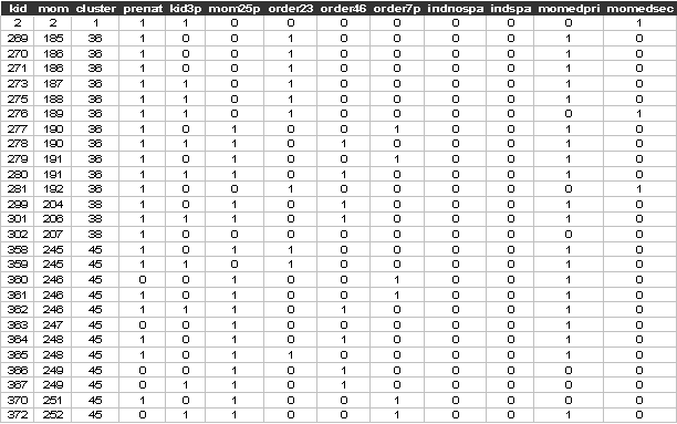
The first few lines and variables of guatemala_prenat.dat look like:

Sabre
commands
out guatemala_prenat.log
data kid mom cluster prenat kid3p mom25p order23 order46 order7p indnospa &
indspa momedpri momedsec husedpri husedsec huseddk husprof husagrself &
husagremp husskilled toilet tvnotdaily tvdaily pcind81 ssdist
read guatemala_prenat.dat
case first=mom second=cluster
yvar prenat
constant cons
mass first=36 second=36
fit kid3p mom25p order23 order46 order7p indnospa indspa momedpri momedsec &
husedpri husedsec huseddk husprof husagrself husagremp husskilled &
toilet tvnotdaily tvdaily pcind81 ssdist cons
dis m
dis e
stop
Sabre
log file
<S> data kid mom cluster prenat kid3p mom25p order23 order46 order7p indnospa &
<S> indspa momedpri momedsec husedpri husedsec huseddk husprof husagrself &
<S> husagremp husskilled toilet tvnotdaily tvdaily pcind81 ssdist
<S> read guatemala_prenat.dat
2449 observations in dataset
<S> case first=mom second=cluster
<S> yvar prenat
<S> constant cons
<S> mass first=36 second=36
<S> fit kid3p mom25p order23 order46 order7p indnospa indspa momedpri momedsec &
<S> husedpri husedsec huseddk husprof husagrself husagremp husskilled &
<S> toilet tvnotdaily tvdaily pcind81 ssdist cons
Initial Homogeneous Fit:
Iteration Log. lik. Difference
__________________________________________
1 -1697.5174
2 -1361.0935 336.4
3 -1348.8843 12.21
4 -1348.6392 0.2450
5 -1348.6389 0.3572E-03
6 -1348.6389 0.1459E-08
Iteration Log. lik. Step End-points Orthogonality
length 0 1 criterion
________________________________________________________________________
1 -1201.2862 1.0000 fixed fixed 16.583
2 -1099.4599 1.0000 fixed fixed 2.3966
3 -1072.8791 1.0000 fixed fixed 1.6688
4 -1060.9384 1.0000 fixed fixed 0.76140
5 -1058.7045 1.0000 fixed fixed 0.36472
6 -1057.4513 0.5000 fixed fixed 2.4320
7 -1056.8794 1.0000 fixed fixed 0.42904
8 -1056.8671 1.0000 fixed fixed 0.38954
9 -1056.8670 1.0000 fixed fixed
<S> dis m
X-vars Y-var Case-var
________________________________________________
cons prenat mom
kid3p cluster
mom25p
order23
order46
order7p
indnospa
indspa
momedpri
momedsec
husedpri
husedsec
huseddk
husprof
husagrself
husagremp
husskilled
toilet
tvnotdaily
tvdaily
pcind81
ssdist
Univariate model
Standard logit
Gaussian random effects
Number of observations = 2449
Number of level 2 cases = 1558
Number of level 3 cases = 161
X-var df = 22
Scale df = 2
Log likelihood = -1056.8670 on 2425 residual degrees of freedom
<S> dis e
Parameter Estimate Std. Err.
___________________________________________________
cons 3.5458 1.7266
kid3p -1.0008 0.30401
mom25p 1.0253 0.52416
order23 -0.70703 0.45506
order46 -0.50441 0.64071
order7p -0.97271 0.84425
indnospa -5.3249 1.5925
indspa -2.8742 1.0720
momedpri 1.8261 0.66167
momedsec 3.9093 1.6070
husedpri 0.80819 0.68186
husedsec 3.4292 1.3501
huseddk 0.57824E-01 1.0320
husprof -0.38402 1.5648
husagrself -1.7913 1.4116
husagremp -2.5822 1.4512
husskilled -0.74278 1.4095
toilet 1.8823 0.95965
tvnotdaily 1.4256 1.3987
tvdaily 1.4827 0.94110
pcind81 -4.5496 1.6165
ssdist -0.50489E-01 0.19281E-01
sclev2 7.0869 0.94235
sclev3 3.6790 0.61058
<S> stop