Example 3LC4. Event history, cloglog link model: time
to fill vacancies of firms (9556 vacancies in 4121 firms)
This is a study of the length of time (level 1, observed at the weekly
level) needed to fill vacancies (level 2) by employers (level 3) in the vacancy
data set vwks4emp_vars.dat. We estimate
a stock model of the duration of the vacancy; in addition to the firm’s
characteristics and those of the vacancy, we use covariates which represent the
stock of the labour market at the current duration, i.e. the total number of
job-seekers (logged) and the total number of vacancies (logged) in the local
labour market.
We use a 10-piece non-parametric baseline hazard
for spell duration (t) with 8 covariates (loguu, logvv, nonman, written, size,
wage, grade, dayrel). Many of the baseline dummy variables coefficients
are similar. The level-2 random effect standard deviation (sclev2) is 1.5825 (SE=0.81508E-01), and the level-3 random
effect standard deviation (sclev3) is 0.82271 (SE=0.55584E-01).
Reference
Andrews, M., Bradley, S., Stott, D., Upward, R., (2007), Testing theories of labour market matching, http://ideas.repec.org/p/ecj/ac2003/209.html
Data
description
Number of observations = 137223 (weeks)
Number of level-2 cases (‘vacref’ = identifier for vacancy) = 9556
Number of level-3 cases (‘empref’ = identifier for firm) = 4121
The variables are:
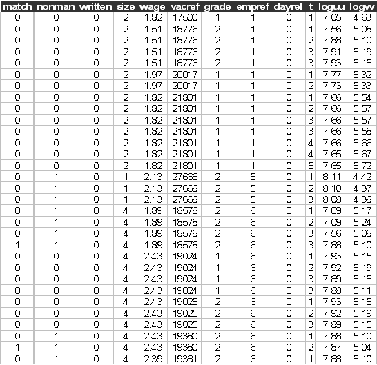
match = 1 if vacancy filled, 0 otherwise in a particular week
nonman = 1 if a non-manual vacancy, 0 otherwise
written = 1 if vacancy required a written method of application, 0 otherwise
size = firm size of the vacancy
wage = log wage of the vacancy
vacref = vacancy reference (a number)
grade = grade required by the vacancy
empref = employer reference (a number)
dayrel = 1 if day release available to the post, 0 otherwise
t = vacancy duration (see below)
loguu = log of stock of job-seekers in the local labour market
logvv = log of stock of vacancies in the local labour market
The covariate (t) for the baseline hazard is defined as follows:
t=1, week 1
t=2, week 2
t=3, weeks 3-4
t=4, weeks 5-6
t=5, weeks 7-8
t=6, weeks 9-13
t=7, weeks 14-26
t=8, weeks 27-39
t=9, weeks 40-52
t=10, weeks 53+
The first few lines and columns of vwks4emp_vars.dat look like:

Sabre
commands
out vwks.log
data match nonman
written size wage vacref grade empref
dayrel t loguu logvv
read /scratch/hpc/22/stott/vwks4emp_vars.dat
case first=vacref second=empref
yvar match
link c
fac t ft
mass first=36 second=36
ari a
fit ft loguu logvv nonman written size wage grade dayrel
dis m
dis e
stop
Sabre
log file
<S>
data match nonman written size wage vacref grade empref dayrel t loguu logvv
<S> read
/scratch/hpc/22/stott/vwks4emp_vars.dat
137223 observations in dataset
<S> case first=vacref second=empref
<S> yvar match
<S> link c
<S> fac t ft
<S> mass first=36 second=36
<S> ari a
<S> fit ft loguu logvv nonman written size wage grade dayrel
Initial Homogeneous Fit:
Iteration Log. lik. Difference
__________________________________________
1 -135728.40
2 -30135.093 0.1056E+06
3 -16451.118 0.1368E+05
4 -12818.836 3632.
5 -11849.767 969.1
6 -11645.414 204.4
7 -11625.888 19.53
8 -11625.385 0.5024
9 -11625.383 0.2028E-02
10 -11625.383 0.6999E-07
Iteration Log. lik. Step End-points Orthogonality
length 0 1 criterion
________________________________________________________________________
1 -11490.967 1.0000 fixed fixed 86.522
2 -11448.769 1.0000 fixed fixed 416.96
3 -11344.893 1.0000 fixed fixed 84.301
4 -11326.158 1.0000 fixed fixed 70.470
5 -11319.106 1.0000 fixed fixed 254.56
6 -11312.097 1.0000 fixed fixed 58.089
7 -11225.904 1.0000 fixed fixed 5.9514
8 -11217.031 1.0000 fixed fixed 4.3284
9 -11216.895 1.0000 fixed fixed 36.100
10 -11216.894 1.0000 fixed fixed 30.277
11 -11216.894 1.0000 fixed fixed
<S> dis m
X-vars Y-var Case-var
________________________________________________
ft match vacref
loguu empref
logvv
nonman
written
size
wage
grade
dayrel
Univariate model
Standard complementary log-log
Gaussian random effects
Number of observations = 137223
Number of level 2 cases = 9556
Number of level 3 cases = 4121
X-var df = 18
Scale df = 2
Log likelihood = -11216.894 on 137203 residual degrees of freedom
<S> dis e
Parameter Estimate Std. Err.
___________________________________________________
ft ( 1) -9.0599 0.57617
ft ( 2) -8.9999 0.56647
ft ( 3) -9.0236 0.56146
ft ( 4) -9.2420 0.56123
ft ( 5) -9.6414 0.56567
ft ( 6) -9.8594 0.56298
ft ( 7) -9.5458 0.56487
ft ( 8) -9.5306 0.57795
ft ( 9) -9.3870 0.59536
ft (10) -9.9367 0.61382
loguu 0.86470 0.63310E-01
logvv -0.73230E-01 0.48542E-01
nonman -0.35115 0.75405E-01
written -0.83641 0.94974E-01
size -0.34307E-01 0.23184E-01
wage -0.17708E-02 0.38449E-01
grade -0.11449 0.42496E-01
dayrel -0.47149 0.95122E-01
sclev2 1.5825 0.81508E-01
sclev3 0.82271 0.55584E-01
<S> stop