Example C1 Continuous
response model
The data we use in this example are a sub-sample from the 1982 High School and Beyond Survey (Raudenbush, Bryk, 2002), and include information on 7,185 students nested within 160 schools: 90 public and 70 Catholic. Sample sizes vary from 14 to 67 students per school.
Reference
Raudenbush, S.W., Bryk, A.S., 2002, Heirarchical
Linear Models,
Data description
Number of observations (rows): 7185
Number of variables (columns): 15
The variables include the following:
school=school identifier
student=student identifier
minority =1 if student is from an ethnic minority,
0 = other)
gender
= 1 if student is female, 0 otherwise
ses = a
standardized scale constructed from variables measuring parental education,
occupation, and income, socio economic status
meanses = mean of the SES values for the students
in this school
mathach=
a measure of the students mathematics achievement
size
= school enrolment
sector
=1 if school is from the Catholic sector,
0 = public
pracad = proportion of students in the academic
track
disclim = a scale measuring disciplinary climate
himnty =1 if more than 40% minority enrolment, 0 if
less than 40%)
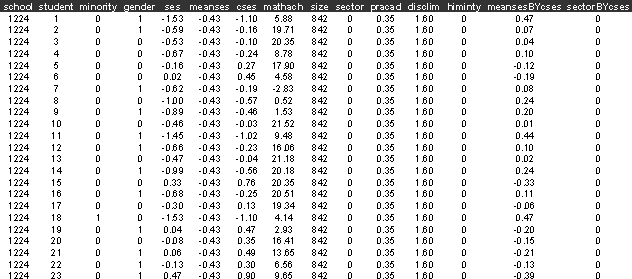
The first few lines of hsb.dat
look like

Sabre commands
out hsb1.log
trace hsb1.trace
data school student minority
gender ses meanses cses mathach size sector &
pracad desclim
himinty meansesbycses sectorbycses
read hsb.dat
case school
yvar mathach
family g
constant cons
lfit
cons
dis m
dis e
mass 64
fit cons
dis m
dis e
lfit meanses cons
dis m
dis e
fit meanses
cons
dis m
dis e
stop
Sabre log file
<S> trace hsb1.trace
<S> data school student minority gender ses meanses
cses mathach size sector
&
<S> pracad desclim himinty meansesbycses sectorbycses
<S> read hsb.dat
7185
observations in dataset
<S> case school
<S> yvar mathach
<S> family g
<S> constant cons
<S> lfit cons
Iteration Log. lik.
Difference
__________________________________________
1 -24049.866
<S> dis m
X-vars Y-var
______________________________
cons mathach
Univariate model
Standard linear
Number of
observations = 7185
X-var df =
1
Log likelihood
= -24049.866 on
7184 residual degrees of freedom
<S> dis e
Parameter Estimate Std. Err.
___________________________________________________
cons
12.748 0.81145E-01
sigma
6.8782
<S> mass 64
<S> fit cons
Initial
Homogeneous Fit:
Iteration Log. lik.
Difference
__________________________________________
1 -24049.866
Iteration Log. lik.
Step End-points Orthogonality
length 0 1
criterion
________________________________________________________________________
1 -23771.600 1.0000 fixed fixed 448.87
2 -23695.571 1.0000 fixed fixed 835.31
3 -23652.804 1.0000 fixed fixed 688.55
4 -23616.853 1.0000 fixed fixed 404.57
5 -23590.245 1.0000 fixed fixed 243.42
6 -23572.704 1.0000 fixed fixed 101.08
7
-23559.124 1.0000 fixed fixed 43.816
8 -23557.935 1.0000 fixed fixed 31.439
9 -23557.905 1.0000 fixed fixed 29.654
10 -23557.905 1.0000 fixed fixed
<S> dis m
X-vars Y-var Case-var
________________________________________________
cons mathach
school
Univariate model
Standard linear
Gaussian random
effects
Number of
observations = 7185
Number of
cases = 160
X-var df =
1
Sigma df =
1
Scale df =
1
Log likelihood
= -23557.905 on
7182 residual degrees of freedom
<S> dis e
Parameter Estimate Std. Err.
___________________________________________________
cons
12.637 0.24359
sigma
6.2569 0.52794E-01
scale 2.9246 0.18257
<S> lfit meanses cons
Iteration Log. lik.
Difference
__________________________________________
1 -23598.190
<S> dis m
X-vars Y-var
______________________________
cons mathach
meanses
Univariate model
Standard linear
Number of
observations = 7185
X-var df =
2
Log likelihood
= -23598.190 on
7183 residual degrees of freedom
<S> dis e
Parameter Estimate Std. Err.
___________________________________________________
cons
12.713 0.76215E-01
meanses 5.7168 0.18429
sigma
6.4596
<S> fit meanses cons
Initial
Homogeneous Fit:
Iteration Log. lik.
Difference
__________________________________________
1 -23598.190
Iteration Log. lik.
Step End-points Orthogonality
length 0 1
criterion
________________________________________________________________________
1 -23502.667 1.0000 fixed fixed 260.90
2 -23489.442 1.0000 fixed fixed 200.22
3 -23483.785 1.0000 fixed fixed 181.86
4 -23481.131 1.0000 fixed fixed 180.44
5 -23480.072 1.0000 fixed fixed 180.76
6 -23479.711 1.0000 fixed fixed 88.600
7 -23479.554 1.0000 fixed fixed 54.074
8 -23479.554 1.0000 fixed fixed 53.557
9 -23479.554 1.0000 fixed fixed
<S> dis m
X-vars Y-var Case-var
________________________________________________
cons mathach
school
meanses
Univariate model
Standard linear
Gaussian random
effects
Number of
observations = 7185
Number of
cases = 160
X-var df =
2
Sigma df =
1
Scale df =
1
Log likelihood
= -23479.554 on 7181 residual degrees of freedom
<S> dis e
Parameter Estimate Std. Err.
___________________________________________________
cons
12.650 0.14834
meanses 5.8629 0.35917
sigma
6.2576 0.52800E-01
scale
1.6103 0.12314
<S> stop