Example C2 Continuous
response model
The data we use in this example are a sub-sample from the 1982 High School and Beyond Survey (Raudenbush, Bryk, 2002), and include information on 7,185 students nested within 160 schools: 90 public and 70 Catholic. Sample sizes vary from 14 to 67 students per school.
Reference
Raudenbush, S.W., Bryk, A.S., 2002, Heirarchical
Linear Models,
Data description
Number of observations (rows): 7185
Number of variables (columns): 15
The variables include the following:
school=school identifier
student=student identifier
minority =1 if student is from an ethnic minority,
0 = other)
gender
= 1 if student is female, 0 otherwise
ses = a
standardized scale constructed from variables measuring parental education,
occupation, and income, socio economic status
meanses = mean of the SES values for the students
in this school
mathach=
a measure of the students mathematics achievement
size
= school enrolment
sector
=1 if school is from the Catholic sector,
0 = public
pracad = proportion of students in the academic
track
disclim = a scale measuring disciplinary climate
himnty =1 if more than 40% minority enrolment, 0 if
less than 40%)
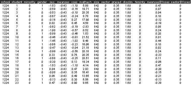
The first few lines of hsb.dat
look like

Sabre commands
out hsb2.log
trace hsb2.trace
data school student minority
gender ses meanses cses mathach size sector &
pracad desclim
himinty meansesbycses sectorbycses
read hsb.dat
case school
yvar mathach
family g
constant cons
lfit
minority gender ses meanses
cons
dis m
dis e
mass 64
fit minority gender ses meanses cons
dis m
dis e
stop
Sabre log file
<S> trace hsb2.trace
<S> data school student minority gender ses meanses
cses mathach size sector
&
<S> pracad desclim himinty meansesbycses sectorbycses
<S> read hsb.dat
7185
observations in dataset
<S> case school
<S> yvar mathach
<S> family g
<S> constant cons
<S> lfit minority gender ses meanses
cons
Iteration Log. lik.
Difference
__________________________________________
1
-23285.328
<S> dis m
X-vars Y-var
______________________________
cons mathach
minority
gender
ses
meanses
Univariate model
Standard linear
Number of
observations = 7185
X-var df =
5
Log likelihood
= -23285.328 on
7180 residual degrees of freedom
<S> dis e
Parameter Estimate Std. Err.
___________________________________________________
cons 14.070 0.11710
minority
-2.3410 0.17381
gender
-1.3200 0.14658
ses 1.9551 0.11151
meanses 2.8675 0.21311
sigma 6.1857
<S> mass 64
<S> fit minority gender ses meanses cons
Initial
Homogeneous Fit:
Iteration Log. lik.
Difference
__________________________________________
1 -23285.328
Iteration Log. lik.
Step End-points Orthogonality
length 0 1
criterion
________________________________________________________________________
1 -23188.269 1.0000 fixed fixed 99.892
2 -23173.011 1.0000 fixed fixed 47.620
3 -23168.722 1.0000 fixed fixed 106.51
4 -23167.251 1.0000 fixed fixed 26.804
5 -23166.850 1.0000 fixed fixed 30.410
6 -23166.721 1.0000 fixed fixed 23.731
7 -23166.634 1.0000 fixed fixed 42.577
8 -23166.634 1.0000 fixed fixed
<S> dis m
X-vars Y-var Case-var
________________________________________________
cons mathach
school
minority
gender
ses
meanses
Univariate model
Standard linear
Gaussian random
effects
Number of
observations = 7185
Number of
cases = 160
X-var df =
5
Sigma df =
1
Scale df =
1
Log likelihood
= -23166.634 on
7178 residual degrees of freedom
<S> dis e
Parameter Estimate Std. Err.
___________________________________________________
cons
14.048 0.17491
minority
-2.7282 0.20412
gender
-1.2185 0.16082
ses 1.9265 0.10844
meanses 2.8820 0.36521
sigma
5.9905 0.50554E-01
scale 1.5480 0.11885
<S> stop