Example FOL1. Depression
in LA
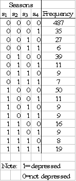
The data in the table below were collected
in a one year panel study of depression and help-seeking behaviour in

However, depression is difficult to overcome suggesting that state dependence might explain at least some of the observed temporal dependence, although it remains an empirical issue whether true contagion extends over three months. We might also expect seasonal effects due to the weather.
References
Morgan,
T.M., Aneshensel, C.S. & Clark, V.A. (1983), Parameter estimation for mover
stayer models: analysis of depression over time, Soc Methods and Research,
11, 345-366.
Conditional analyses
(1) Conditional on the
initial response
Data description (dep_rob2.dat):
The
model for the binary depression data (dep_rob2.dat), ignoring the model for the
initial response, has constant, dummy variables for seasons 3 and 4 and the
lagged response variable.
The
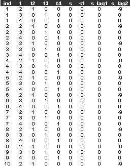
data (dep_rob2.dat) has:
Number
of observations: 2256
Number
of cases: 752
The
variables are:
t=season
t2=1
if t=2, 0 otherwise
t3=1
if t=3, 0 otherwise
t4=1
if t=4, 0 otherwise
s=
binary indicator for depression (1 if yes, 0 otherwise)
s1=baseline
response
s_lag1=lag
1 response
s_lag2=lag
2 response (not used)
The
first few lines of the data set (dep_rob2.dat) look like:

Sabre commands
out depression1.log
data
read dep_rob2.dat
case
yvar s
link p
constant cons
mass 24
fit t3 t4 s_lag1
cons
dis m
dis e
stop
Sabre log file
Log likelihood = -831.56731 on 2251 residual degrees of freedom
Parameter Estimate Std. Err.
___________________________________________________
cons -1.2942 0.72379E-01
t3 -0.15466 0.88638E-01
t4 -0.21480E-01 0.87270E-01
s_lag1 0.94558 0.13563
scale 0.32841 0.18226
The
coefficient on s_lag1 is 0.94558 (s.e. 0.13563), which is
highly significant, but the scale parameter
is of marginal significance, suggesting a nearly homogeneous first order
model. Can we trust this inference?
(2) Condition on the initial response but allow
the random effect to be dependent on initial response and time constant
covariates,
Wooldridge (2005)
The
model for the binary depression data (dep_rob2.dat), ignoring the model for the
initial response, has constant, dummy variables for seasons 3 and 4, the lagged
response variable and the initial response.
References
Wooldridge, J.M., (2005), Simple solutions to the initial
conditions problem in dynamic, nonlinear panel data models with unobserved
heterogeneity, Journal of Applied
Econometrics, 20, 39---54.
Sabre
commands
out depression1b.log
data
read dep_rob2.dat
case
yvar s
link p
constant cons
mass 24
fit t3 t4 s_lag1
s1 cons
dis m
dis e
stop
Gives
Log likelihood = -794.75310 on 2250 residual degrees of freedom
Parameter Estimate Std. Err.
___________________________________________________
cons -1.6646 0.11654
t3 -0.20988 0.99663E-01
t4 -0.88079E-01 0.97569E-01
s_lag1 0.43759E-01 0.15898
s1 1.2873 0.19087
scale 0.88018 0.12553
This
has the lagged response s_lag1 estimate at 0.43759E-01 (0.15898), which is not
significant, while the initial response s1 estimate 1.2873 (0.19087) and the
scale parameter estimate 0.88018 (0.12553) are highly significant. There is
also a big improvement in the log-likelihood over the model without s1 of 73.63 for 1 df. This model has no time-constant
covariates to be confounded by the auxiliary model and suggests that depression
is a zero order process.
Modelling the initial conditions (joint
analysis)
There
are several approximations that can be adopted: (1) use the same random effect
in the initial and subsequent responses, e.g. Crouchley and Davies (2001); (2)
use a one-factor decomposition for the initial and subsequent responses, e.g.
Heckman (1981a), Stewart (2007); (3) use different (but correlated) random
effects for the initial and subsequent responses; (4) embed the Wooldridge
(2005) approach in joint models for the initial and subsequent responses.
References
Crouchley, R., & Davies, R.B., (2001), A comparison of
GEE & random effects models for distinguishing hetero-geneity,
nonstationarity & state dependence in a collection of short binary event
series, Stat Mod, 1, 271-285.
Heckman
J.J., (1981a), Statistical models for discrete panel data, In Manski, C.F.
& McFadden, D, (eds), Structural
analysis of discrete data with econometric applications, MIT press,
Stewart, M.B., (2007), The interrelated dynamics of
unemployment and low-wage employment
Journal of
Applied Econometrics, Volume 22, 511-531
Wooldridge, J.M., (2005), Simple solutions to the initial
conditions problem in dynamic, nonlinear panel data models with unobserved
heterogeneity, Journal of Applied
Econometrics, 20, 39---54.
(1) Same random effect in the initial and
subsequent responses with a common scale parameter
The
joint model for the binary depression data (depression.dat) has a constant for
the initial response, a constant for the subsequent responses, dummy variables
for seasons 3 and 4 and the lagged response variable.
Data
description
Number
of observations: 3008
Number
of cases: 752
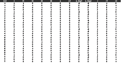
The
variables are:
t=season
(1,2,3,4)
t1=1
if t=1, 0 otherwise
t2=1
if t=2, 0 otherwise
t3=1
if t=3, 0 otherwise
t4=1
if t=4, 0 otherwise
s=
binary indicator for depression (1 if yes, 0 otherwise)
s1=baseline
response
s_lag1=lag
1 response, -9 if missing
s_lag2=lag
2 response, -9 if missing (not used)
r=response
position, 1 if baseline, 2 if subsequent response
r1=1
if r=1, 0 otherwise
r2=1
if r=2, 0 otherwise
The
first few lines of the data set (depression.dat) look like:

In
the depression example, the model for the initial response (indicator r1=1),
has only a constant, the model for the 3 subsequent responses (indicator r2=1)
has a constant, dummy variables for seasons 3 (r2_t3 ) and 4 (r2_t4), and the
lagged response variable(r2_lag1).
Sabre commands
out depression2.log
data
read depression.dat
case
yvar s
link p
trans r2_t3 r2 *
t3
trans r2_t4 r2 *
t4
trans r2_lag1 r2 * s_lag1
mass 24
fit r1 r2 r2_t3
r2_t4 r2_lag1
dis m
dis e
stop
Gives
Log likelihood = -1142.9749 on 3002 residual degrees of freedom
Parameter Estimate Std. Err.
___________________________________________________
r1 -1.3476 0.10026
r2 -1.4708 0.92548E-01
r2_t3 -0.20740 0.99001E-01
r2_t4 -0.85438E-01 0.97129E-01
r2_lag1 0.70228E-01 0.14048
scale 1.0372 0.10552
The
coefficient of r2_lag1 is 0.70228E-01 (0.14048) suggesting that there is no
state dependence in these data, while the scale coefficient 1.0372 (0.10552)
suggests heterogeneity.
(2) Same random effect in the initial and
subsequent responses but with different scale parameters
As
in the common scale parameter model, the joint model for the binary depression
data (depression.dat) has a constant for the initial response, a constant for
the subsequent responses, dummy variables for seasons 3 and 4 and the lagged
response variable.
Sabre
commands
out depression3.log
data
read depression.dat
case
yvar s
rvar r
link p
trans r2_t3 r2 *
t3
trans r2_t4 r2 *
t4
trans r2_lag1 r2 *
s_lag1
mass 24
depend y
nvar 1
fit r1 r2 r2_t3
r2_t4 r2_lag1
dis m
dis e
stop
Gives
Log likelihood = -1142.9355 on 3001 residual degrees of freedom
Parameter Estimate Std. Err.
___________________________________________________
r1 -1.3248 0.12492
r2 -1.4846 0.10639
r2_t3 -0.21020 0.10004
r2_t4 -0.87882E-01 0.98018E-01
r2_lag1 0.50254E-01 0.15792
scale1 1.0021 0.15927
scale2 1.0652 0.14587
This
shows that the state dependence regressor r2_lag1 has estimate 0.50254E-01
(0.15792), which is not significant. It also shows that the scale parameters
are nearly the same. The log likelihood improvement of the model with 2 scale
parameters over that of the previous model with 1 scale parameter is 0.079 for 1 df. Thus the model with 1 scale
parameter is to be preferred.
(3) Different random effects in the initial and
subsequent responses
As
in the single random effect models, the joint model for the binary depression
data (depression.dat) has a constant for the initial response, a constant for
the subsequent responses, dummy variables for seasons 3 and 4 and the lagged
response variable.
Sabre
commands
out depression4.log
data
data
read depression.dat
case
yvar s
model b
rvar r
link first=p second=p
trans r2_t3 r2
* t3
trans r2_t4 r2
* t4
trans r2_lag1 r2 * s_lag1
mass first=24
second=24
eqscale y
der1 y
nvar 1
fit r1 r2
r2_t3 r2_t4 r2_lag1
dis m
dis e
stop
Gives
Log likelihood = -1142.9355 on 3001 residual degrees of freedom
Parameter Estimate Std. Err.
___________________________________________________
r1 -1.3672 0.12386
r2 -1.4846 0.10591
r2_t3 -0.21020 0.10033
r2_t4 -0.87881E-01 0.97890E-01
r2_lag1 0.50253E-01 0.15946
scale 1.0652 0.14362
corr 0.97091 0.10087
Note
that the log likelihood is exactly the same as for the previous model, the
scale2 parameter from the previous model has the same value as the scale
parameter of the current model. The lagged response r2_lag1 has an estimate of
0.50313E-01 (0.15945), which is not significant. The correlation between the
random effects (corr) has estimate 0.97089 (0.10093), which is very close to 1
suggesting that the common random effects, zero order, single scale parameter
model is to be preferred.
(4) Embed the Wooldridge (2005) approach in
joint models for the initial and subsequent responses
As
in the single random effect models, the joint model for the binary depression
data (depression.dat) has a constant for the initial response, a constant for
the subsequent responses, dummy variables for seasons 3 and 4, the lagged
response variable and the initial response variable.
Sabre
commands
out depression5.log
data
read depression.dat
case
yvar s
link p
trans r2_t3 r2 *
t3
trans r2_t4 r2 *
t4
trans r2_lag1 r2 * s_lag1
trans r2_base r2 *
s1
mass 24
fit r1 r2 r2_t3
r2_t4 r2_lag1 r2_base
dis m
dis e
stop
Gives
Log likelihood = -1142.9670 on 3001 residual degrees of freedom
Parameter Estimate Std. Err.
___________________________________________________
r1 -1.3632 0.16189
r2 -1.4741 0.97129E-01
r2_t3 -0.20869 0.99797E-01
r2_t4 -0.86541E-01 0.97774E-01
r2_lag1 0.61490E-01 0.15683
r2_base -0.33544E-01 0.26899
scale 1.0602 0.21274
This
joint model has both the lagged response r2_lag1 estimate of 0.61490E-01
(0.15683) and the baseline/initial response effect r2_base estimate of
-0.33544E-01 (0.26899) as being non-significant.
If
we estimate a standard zero order model with dummy variables for seasons 2, 3,
and 4 to all the data we get
Parameter Estimate Std. Err.
___________________________________________________
cons -1.3712 0.90331E-01
t2 -0.10411 0.94043E-01
t3 -0.31491 0.98105E-01
t4
-0.19507 0.95630E-01
scale 1.0734 0.78059E-01
This
model, without any state dependence, suggests that the worst seasons are t3
(autumn) and t4 (winter). This model also has a good fit to the data, the log
L(Data)=-1141.54, so the ChiSq (goodness of fit to the data) is 3.11 with 10 df.