Example L2 Continuous
response model
We analyses a version of the NLSY data as used in various Stata Manuals (to illustrate the xt commands). The data is for young women who were aged 14-26 in 1968. The women were surveyed each year from 1970 to 1988, except for 1974, 1976, 1979, 1981, 1984 and 1986. We have removed records with missing values on one or more of the response and explanatory variables we want use in our analysis of the joint determinants of wages and trade union membership. In this example we model the wage response. There are 4132 women (idcode) with between 1 and 12 years of observation on wages being in employment (i.e. not in full time education) and earning more than $1/hour but less than $700/hour.
Reference
Stata Longitudinal/Panel Data,
Reference Manual, Release 9, (2005), Stata Press, StataCorp LP,
Data description
Number of observations (rows): 18995
Number of variables (columns): 20
The subset of variables we use are:
ln_wage=ln(wage/GNP deflator) in a particular year are:
black=1 if woman is black, 0 otherwise;
msp=1 if woman is married and spouse is present, 0 otherwise;
grade= years of schooling completed; (0-18);
not_smsa=1 if woman was living outside a standard metropolitan statistical area (smsa), 0 otherwise;
south=1 if the woman was living in the South, 0 otherwise;
union=1 if a member of a trade union, 0 otherwise;
tenure= job tenure in years (0-26).
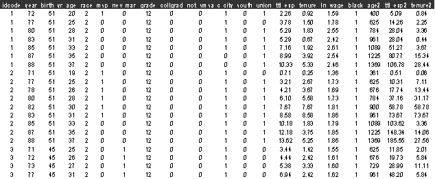
The first few lines of nls.dat
look like

Sabre commands
out wage.log
trace wage.trace
data idcode
year birth_yr age race msp nev_mar grade collgrad not_smsa &
c_city south union ttl_exp tenure ln_wage black age2
ttl_exp2 tenure2
read nls.dat
case idcode
yvar ln_wage
family g
constant cons
lfit
black msp grade not_smsa
south union tenure cons
dis m
dis e
mass 64
fit black msp
grade not_smsa south union tenure cons
dis m
dis e
stop
Sabre log file
<S> trace wage.trace
<S> data idcode year birth_yr age race msp nev_mar grade collgrad not_smsa &
<S> c_city south union ttl_exp tenure
ln_wage black age2 ttl_exp2 tenure2
<S> read nls.dat
18995
observations in dataset
<S> case idcode
<S> yvar ln_wage
<S> family g
<S> constant cons
<S> lfit black msp grade not_smsa south union
tenure cons
Iteration Log. lik. Difference
__________________________________________
1 -8329.7229
<S> dis m
X-vars Y-var
______________________________
cons ln_wage
black
msp
grade
not_smsa
south
union
tenure
Univariate model
Standard linear
Number of
observations = 18995
X-var df =
8
Log likelihood
= -8329.7229 on
18987 residual degrees of freedom
<S> dis e
Parameter Estimate Std. Err.
___________________________________________________
cons
0.82027 0.16614E-01
black
-0.10093 0.66150E-02
msp 0.50526E-03 0.57363E-02
grade 0.69701E-01 0.11861E-02
not_smsa
-0.18494
0.62495E-02
south
-0.80056E-01 0.59837E-02
union
0.13725 0.66379E-02
tenure
0.32222E-01 0.67368E-03
sigma
0.37523
<S> mass 64
<S> fit black msp grade not_smsa south union tenure cons
Initial
Homogeneous Fit:
Iteration Log. lik.
Difference
__________________________________________
1 -8329.7229
Iteration Log. lik.
Step End-points Orthogonality
length 0 1
criterion
________________________________________________________________________
1 -9467.6528 1.0000 fixed fixed 2046.9
2 -8984.0889 1.0000 fixed fixed 913.78
3 -7780.0804 1.0000 fixed fixed 2743.7
4 -5809.8772 0.5000
fixed fixed 17164.
5 -5329.1065 0.5000 fixed fixed 0.16462E+06
6 -5128.8993 1.0000 fixed fixed 0.12681E+06
7 -4938.3977 1.0000 fixed fixed 0.41150E+06
8 -4871.7215 1.0000 fixed fixed 0.34215E+06
9 -4870.4148 1.0000 fixed fixed 0.34370E+06
10 -4870.4141 1.0000 fixed fixed 0.35343E+06
11 -4870.4141 1.0000 fixed fixed
<S> dis m
X-vars Y-var Case-var
________________________________________________
cons ln_wage idcode
black
msp
grade
not_smsa
south
union
tenure
Univariate model
Standard linear
Gaussian random
effects
Number of
observations = 18995
Number of
cases = 4132
X-var df =
8
Sigma df =
1
Scale df =
1
Log likelihood
= -4870.4141 on
18985 residual degrees of freedom
<S> dis e
Parameter Estimate Std. Err.
___________________________________________________
cons
0.76119 0.27736E-01
black
-0.77839E-01 0.11567E-01
msp -0.38486E-02 0.58172E-02
grade
0.72769E-01 0.20097E-02
not_smsa
-0.14126
0.87666E-02
south
-0.74745E-01 0.85956E-02
union
0.11106 0.64703E-02
tenure
0.28474E-01 0.63994E-03
sigma
0.26019 0.15142E-02
scale
0.27966 0.40104E-02
<S> stop