Example L3 Continuous
response growth model
Snijders & Bosker, (1999) analysed the
development over time of teacher evaluations. Starting from the first year of their career,
teachers were evaluated on their interpersonal behaviour in the classroom. This happened repeatedly, at intervals of
about one year. In this example, results
are presented about the 'proximity' dimension, representing the degree of
cooperation or closeness between a teacher and his or her students. The higher the proximity score of a teacher,
the more cooperation is perceived by his or her students.
There are four measurement occasions: after 0, 1, 2, and 3
years of experience. A total of 51
teachers were studied. The number of observations for the 4 moments decreased
from 46 at time i=0 to 32 at time i=3. The non-response at various is treated as
ignorable.
Reference
Snijders, T. A. B. and Bosker, R. J. (1999). Multilevel
Analysis.
Data description
Number of observations (rows): 153
Number of variables (columns): 8
The subset of variables we use are:
teacher = teacher identifier
time = 0,1,2,3 the year at which the teacher evaluation was made
proximity = degree of cooperation or closeness between a teacher and his or her students
gender = 1 if teacher is female, 0 otherwise
d1 = 1 if time =0, 0 otherwise
d2 = 1 if time =1, 0 otherwise
d3 = 1 if time =2, 0 otherwise
d4 = 1 if time =3, 0 otherwise
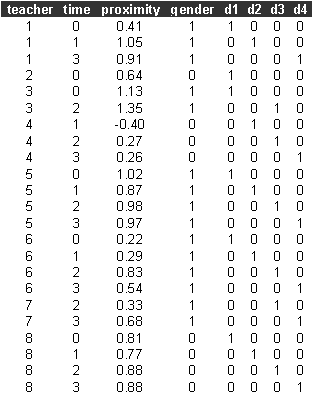
The first few lines of growth.dat look like

Sabre commands
out growth.log
trace growth.trace
data teacher time proximity gender d1 d2 d3 d4
read growth.dat
case teacher
yvar proximity
family g
constant cons
lfit cons
dis m
dis e
mass 64
scale 0.5
fit cons
dis m
dis e
lfit d1 d2 d3 d4
dis m
dis e
sigma 0.25
scale 0.5
fit d1 d2 d3 d4
dis m
dis e
stop
Sabre log file
<S> trace growth.trace
<S> data teacher time proximity gender d1 d2 d3 d4
<S> read growth.dat
153
observations in dataset
<S> case teacher
<S> yvar proximity
<S> family g
<S> constant cons
<S> lfit cons
Iteration Log. lik. Difference
__________________________________________
1 -88.715008
<S> dis m
X-vars Y-var
______________________________
cons proximity
Univariate
model
Standard linear
Number of
observations = 153
X-var df =
1
Log likelihood
= -88.715008 on
152 residual degrees of freedom
<S> dis e
Parameter Estimate Std. Err.
___________________________________________________
cons 0.63856 0.35048E-01
sigma 0.43352
<S> mass 64
<S> scale 0.5
<S> fit cons
Initial
Homogeneous Fit:
Iteration Log. lik. Difference
__________________________________________
1 -88.715008
Iteration Log. lik. Step End-points Orthogonality
length 0 1
criterion
________________________________________________________________________
1 -84.581007 1.0000 fixed
fixed 136.94
2 -75.772623 0.5000 fixed
fixed 1298.9
3 -64.493890 1.0000 fixed
fixed 741.33
4 -61.916672 1.0000 fixed
fixed 606.92
5 -61.737341 1.0000 fixed
fixed 1198.4
6 -61.702731 1.0000 fixed
fixed 661.65
7 -61.688023 1.0000 fixed
fixed 1557.1
8 -61.688018 1.0000 fixed
fixed 1843.3
9 -61.688018 1.0000 fixed
fixed
<S> dis m
X-vars Y-var Case-var
________________________________________________
cons proximity teacher
Univariate
model
Standard linear
Gaussian random
effects
Number of
observations = 153
Number of
cases = 51
X-var df =
1
Sigma df =
1
Scale df =
1
Log likelihood
= -61.688018 on
150 residual degrees of freedom
<S> dis e
Parameter Estimate Std. Err.
___________________________________________________
cons 0.64795 0.53346E-01
sigma 0.27155 0.19025E-01
scale 0.34388 0.42213E-01
<S> lfit d1 d2 d3 d4
Iteration Log. lik. Difference
__________________________________________
1 -87.536537
<S> dis m
X-vars Y-var
______________________________
d1 proximity
d2
d3
d4
Univariate
model
Standard linear
Number of
observations = 153
X-var df =
4
Log likelihood
= -87.536537 on
149 residual degrees of freedom
<S> dis e
Parameter Estimate Std. Err.
___________________________________________________
d1 0.58652 0.64064E-01
d2 0.72395 0.70485E-01
d3 0.64378 0.71431E-01
d4 0.60594 0.76810E-01
sigma 0.43450
<S> sigma 0.25
<S> scale 0.5
<S> fit d1 d2 d3 d4
Initial
Homogeneous Fit:
Iteration Log. lik. Difference
__________________________________________
1 -87.536537
Iteration Log. lik. Step End-points Orthogonality
length 0 1
criterion
________________________________________________________________________
1 -64.095200 1.0000 fixed
fixed 94.548
2 -63.262786 0.5000 fixed
fixed 773.48
3 -60.084462 1.0000 fixed
fixed 507.61
4 -59.421825 1.0000 fixed
fixed 182.88
5 -59.263588 1.0000 fixed
fixed 310.69
6 -59.204119 1.0000 fixed
fixed 204.81
7 -59.146517 1.0000 fixed
fixed 335.13
8 -59.146452 1.0000 fixed
fixed 348.43
9 -59.146452 1.0000 fixed
fixed
<S> dis m
X-vars Y-var Case-var
________________________________________________
d1 proximity teacher
d2
d3
d4
Univariate
model
Standard linear
Gaussian random
effects
Number of
observations = 153
Number of
cases = 51
X-var df =
4
Sigma df =
1
Scale df =
1
Log likelihood
= -59.146452 on
147 residual degrees of freedom
<S> dis e
Parameter Estimate Std. Err.
___________________________________________________
d1 0.58508 0.62624E-01
d2 0.71760 0.66132E-01
d3 0.67158 0.66631E-01
d4 0.63893 0.69505E-01
sigma 0.26500 0.18573E-01
scale 0.34532 0.41967E-01
<S> stop