Example L5 Ordered
response model
In this example we analyse ordinal data on changes in the severity of Schizophrenia in data from the National Institute of Mental Health (NIMH), see Rabe-Hesketh and Skrondal (2005, Ch 5). Patients were randomly allocated to 1 of 4 treatments (Placebo, Chlorpromazine, Fluphenazine, Thioridazine) and examined weekly for up to 6 weeks. The data have previously been analysed by Hedeker and Gibbons (1996a), Gibbons et al. (1998) and Gibbons and Hedeker (1994). In this example we follow Rabe-Hesketh and Skrondal (2005, Ch 5) and combine the treatments Chlorpromazine, Fluphenazine and Thioridazine.
Data description
Number of observations (rows): 1603
Number of variables (columns): 8
Variables:
id=subject identifier
week=week (0,1,2,…,6) of assessment since randomisation to treatment;
imps=score on item 79 of the Inpatient Multidimensional Psychiatric Scale (IMPS) of Lorr and Klextt (1966).
treatment=1 if subject was in the treatment group (drug), 0 otherwise;
Following Rabe-Hesketh and Skrondal (2005, Ch 5) and Hedeker and Gibbons (1996a) we recode the imps variable into impso, an ordinal variable with 4 categories, i.e.
impso=1 if 1<=imps<=2.4;
impso=2 if 2.5<=imps<4.4
impso=3 if 4.5<=imps<=5.4
impso=4 if 5.5<=imps<=7
Following Rabe-Hesketh and Skrondal (2005, Ch 5) we also use the square root of week (weeksqrt) instead of week in its raw form as an explanatory variable. Similarly we also produce a new variable from the interaction (interact) of weeksqrt and treatment.
References
Gibbons, R. D., Hedeker, C., Waterneaux, C., & Davis, J.M., (1988), Random regression models: A comprehensive approach to the analysis of longitudinal psychiatric data, Psychopharmacology Bulletin, 24, 438-443
Gibbons, R. D., & Hedeker, C., (1994), Application of random effects probit regression models, Journal of Consulting and Clinical Psyschology.
Hedeker, D., & Gibbons, R.D., (1996), Applied
longitudinal data anlaysis,
Rabe-Hesketh, S., and Skrondal, A., (2005), Multilevel and Longitudinal Modelling using Stata, Stata Press, Stata Corp, College Station, Texas.
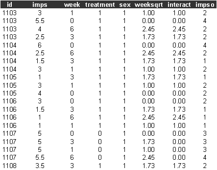
The first few lines of schiz.dat look like

Sabre commands
out schiz.log
trace schiz.trace
data id imps week treatment sex weeksqrt interact impso
read schiz.dat
case id
yvar impso
ordered y
lfit weeksqrt treatment interact
dis m
dis e
fit weeksqrt treatment interact
dis m
dis e
stop
Sabre log file
<S> trace schiz.trace
<S> data id imps week treatment sex weeksqrt
interact impso
<S> read schiz.dat
1603
observations in dataset
<S> case id
<S> yvar impso
<S> ordered y
<S> lfit weeksqrt treatment interact
Iteration Log. lik. Step End-points Orthogonality
length 0 1
criterion
________________________________________________________________________
1 -2239.6731 1.0000 fixed
fixed 18.971
2 -1947.5622 0.5000 fixed
fixed 46.248
3 -1885.7509 1.0000 fixed
fixed 131.39
4 -1879.9699 1.0000 fixed
fixed 248.84
5 -1878.6522 1.0000 fixed
fixed 1158.2
6 -1878.2740 1.0000 fixed
fixed 253.33
7 -1878.0969 1.0000 fixed
fixed 54.836
8 -1878.0969 1.0000 fixed
fixed
<S> dis m
X-vars Y-var
______________________________
weeksqrt impso
treatment
interact
Univariate
model
Standard
ordered logit
Number of
observations = 1603
X-var df =
3
Log likelihood
= -1878.0969 on
1600 residual degrees of freedom
<S> dis e
Parameter Estimate Std. Err.
___________________________________________________
weeksqrt -0.53665 0.11081
treatment -0.60428E-03 0.18833
interact -0.75097 0.12768
cut1 -3.8073 0.18986
cut2 -1.7602 0.17027
cut3 -0.42211 0.16363
<S> fit weeksqrt treatment interact
Initial
Homogeneous Fit:
Iteration Log. lik. Step End-points Orthogonality
length 0 1
criterion
________________________________________________________________________
1 -2239.6731 1.0000 fixed
fixed 18.971
2 -1947.5622 0.5000 fixed
fixed 46.248
3 -1885.7509 1.0000 fixed
fixed 131.39
4 -1879.9699 1.0000 fixed
fixed 248.84
5 -1878.6522 1.0000 fixed
fixed 1158.2
6 -1878.2740 1.0000 fixed
fixed 253.33
7 -1878.0969 1.0000 fixed
fixed 54.836
8 -1878.0969 1.0000 fixed
fixed
Iteration Log. lik. Step End-points Orthogonality
length 0 1
criterion
________________________________________________________________________
1 -1775.2726 1.0000 fixed
fixed 14.707
2 -1717.2806 1.0000 fixed
fixed 12.350
3 -1703.2212 1.0000 fixed
fixed 119.24
4 -1701.5195 1.0000 fixed
fixed 340.03
5 -1701.2283 1.0000 fixed
fixed 337.78
6 -1701.1745 1.0000 fixed
fixed 211.94
7 -1701.1622 1.0000 fixed
fixed 18.610
8 -1701.1622 1.0000 fixed
fixed
<S> dis m
X-vars Y-var Case-var
________________________________________________
weeksqrt impso id
treatment
interact
Univariate
model
Standard
ordered logit
Gaussian random
effects
Number of
observations = 1603
Number of
cases = 437
X-var df =
3
Scale df =
1
Log likelihood
= -1701.1622 on
1599 residual degrees of freedom
<S> dis e
Parameter Estimate Std. Err.
___________________________________________________
weeksqrt -0.76775 0.13107
treatment -0.81896E-01 0.31086
interact -1.2069 0.15280
cut1 -5.8917 0.33345
cut2 -2.8572 0.28969
cut3 -0.73532 0.27343
scale 1.9520 0.12113
<S> stop