Exercise FOL2 Probit model of union membership of females, Stewart (2006)
This exercise uses the union data for US young
women from the National Longitudinal Survey of Youth (NLSY) from the Stata manual
(http://www.stata-press.com/data/r9/union.dta). We use the same subsample that was used by Stewart (2006) to illustrate his
Stata program (redprob). To
form this subsample Stewart (2006) uses only data
from 1978 onwards; the data for 1983 are dropped, and only those individuals
observed in each of the remaining 6 waves are kept. This gave a balanced panel
with N = 799 individuals observed in each of 6 waves. The observations for 1985
and 1987 are implicitly treated as if they were for 1984 and 1986 respectively,
which would give 6 waves at regular 2-year intervals. Trade union membership is
determined by the question of whether of not the sampled individual had her
wage set in a collective bargaining agreement or not.
References
Stewart, M.B., (2006), -redprob-
A Stata program for the Heckman estimator of the
random effects dynamic probit model,
http://www2.warwick.ac.uk/fac/soc/economics/staff/faculty/stewart/stata/redprobnote.pdf
Conditional analysis
Data description
(unionred1.dat)
Number of observations = 3995
Number of cases = 799
The variables include the following:
idcode=NLSY subject identifier code
year=interview
year
age=age
in current year
grade=years
of schooling completed
not_smsa=1
if living outside a standard metropolitan statistical area, 0 otherwise
south=1
if south, 0 otherwise
union=1
if wage is collectively negotiated, 0 otherwise
t0= year-70
southXt=1 if resident in south, 0 otherwise
black=1
if race black, 0 otherwise
tper=panel wave
lagunion=the value of union in the previous interval
d=2 for all responses, as all responses are post
baseline.
d1=0 for all responses, as all responses are post
baseline
d2=1 for all responses, as all responses are post
baseline
baseunion=1 if union=1 in 1978, 0 otherwise
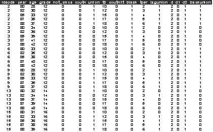
The first few rows and columns of unionred1.dat
look like

Exercise
1)
Estimate a heterogeneous probit
(level-2 with idcode, mass 24) model of trade union
membership (union), with a constant and the lagged union membership variable (lagunion), age, grade, and southXt
regressors.
2)
Add the initial condition of trade union membership
in 1978 (baseunion) to the previous model. How does the inference on the lagged response (lagunion) and the scale effects differ between the two
models.
Joint analysis of the
initial condition and subsequent responses
Data description (unionred.dat)
Number of observations = 4794
Number of cases = 799
The variables are the same as unionred1.dat except
that this time the variables
d, d1 and d2
take more values.
d=1, for the initial response, 2 if a subsequent
response
d1=1 if d=1, 0 otherwise
d2=1 if d=2, 0 otherwise
The first few rows and columns of unionred.dat look like

Exercise
1)
Estimate a common random effect common scale joint probit model (mass 24) of trade union membership (union).
Use constants in both linear predictors. Use the d1 and d2 dummy variables to
set up the linear predictors. For the initial response use the regressors: age, grade, southXt
and not_smsa. For the subsequent response use the regressors: lagged union membership variable (lagunion), age, grade, southXt.
What does this model suggest about state dependence and unobserved
heterogeneity?
2)
Re-estimate the model allowing the scale parameters
for the initial and subsequent responses to be different. Is this a significant
improvement over the common scale parameter model?
3)
To the different scale model add the initial or
baseline response (baseunion). Does this make a
significant improvement to the model?