Exercise FOL3 Binary
Response, Female Labour Force Participation in the
Davies, Elias and Penn (1992) and Davies (1993) as
part of the ESRC funded Social Change and Economic Life Initiative. The data we
use is the annual employment behaviour of wives from Rochdale (UK) from the
date of their marriage to the end of the survey in 1987. The binary response femp takes the value 1 if a wife was employed in the current
year and 0 otherwise. There is a set of explanatory variables that include
husband's employment status and age (years). In this exercise we are going to
see if we can distinguish state dependence (first order effects) in employment
behaviour of wives from unobserved heterogeneity. The same data (wemp.dta) were used by Rabe-Hesketh
and Skrondal (2005, exercise 4.5).
References
Davies, R.B., Elias, P., and Penn, R., (1992), The relationship between a husband's unemployment and his
wife's participation in the labour force, Oxford Bulletin of Economics and
Statistics, 54, 145-171
Davies, R.B., (1993), Statistical modelling for
survey analysis, Journal of the Market Research Society, 35, 235-247.
Rabe-Hesketh,
S., & Skrondal, A., (2005), Multilevel and Longitudinal
Modelling using Stata, Stata
Press, Stata Corp, College Station, Texas
Conditional analysis
Data description
(wemp_base2.dat)
Number of observations = 1274
Number of cases = 144
The variables include the following:
case=
identifier for wives
femp=1 if wife is in employment status in current year,
0 otherwise
mune=1 if the husband is in employment in current year,
0 otherwise
time=year
of observation-1975
und1=1 if the wife has children under the age of 1,
0 otherwise
und5=1 if the wife has children under the age of 5,
0 otherwise
age=wife's
age-1975
d=1 if mmmmmm, 2
otherwise?
d1=1 if d=1, 0 otherwise
d0=1 if d=2, 0 otherwise
ylag=femp
lagged 1 year
ybase=femp in
1st year
r=2 for all post 1st year observations
r1=0 for all observations
r2=1, if r=2
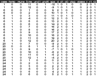
The first few lines of wemp_base2.dat look like:

Exercise
1)
Estimate a heterogeneous logit
(level-2 with case, mass 20) model of female employment participation (femp), with a constant and the lagged female employment
participation variable (ylag), mune,
und5, and age regressors.
2)
Add the initial condition of employed in the 1st
year (ybase) to the previous model. How do the
inference on the lagged responses (ylag) and the
scale effects differ between the two models.
Joint analysis of the
initial condition and subsequent responses
Data description (wemp_base.dat)
Number of observations = 1425
Number of cases = 151
The variables are the same as wemp_base2.dat except
that this time the variables ylag, r, r1 and r2 take
more values.
ylag=femp
lagged 1 year, -9 if its the 1st year
r=1, for the initial response, 2 if a subsequent
response
r1=1 if d=1, 0 otherwise
r2=1 if d=2, 0
otherwise
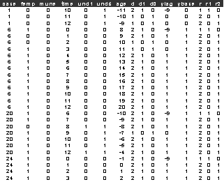
The first few rows of wemp_base.dat
look like

Exercise
1)
Estimate a common random effect common scale joint logit model (mass 20) of female employment participation (femp). Use constants in both linear predictors. Use the d1
and d2 dummy variables to set up the linear predictors. For the initial
response use the regressors: mune,
und5, and age regressors. For the subsequent
responses use the regressors: the lagged female
employment participation variable (ylag), mune, und5, and age. What does this model suggest about
state dependence and unobserved heterogeneity?
2)
Re-estimate the model using a bivariate
model for the random effects (common scale). What is the value of rho? Is this a significant improvement over the common
scale parameter model?
3)
To the bivariate model
add the initial or baseline response (ybase). Does
this make a significant improvement to the model?
4)
Compare the results obtained for the various models
on the covariates and role of employment status in the previous year. Are both
state dependence and unobserved heterogeneity present in this data? Do the
results on the covariates make intuitive sense?