Exercise L10, bivariate model, linear and binary
Vella and Verbeek (1998) analysed the male data from the Youth Sample of the US National Longitudinal Survey for the period 1980-1987. The number of young males in the sample is 545. The version of the data set (wagepan.dat) we use was obtained from Wooldridge (2002). The same data were used for modelling the wages and for separately modelling trade union membership by Rabe-Hesketh and Skrondal (2005, exercises 2.7 and 4.7). We start by re-estimating the separate models for log(wages) and for trade union membership. We then estimate a joint model thus allowing trade union membership to be endogenous in the wage equation.
Data description
Number of observations (rows): 4360
Number of variables (columns): 44
Description of the sub-set of variables we are going to use in this exercise:
nr= person identifier
year=1980 to 1987
black=1 if respondent is black,0 otherwise
exper=labour market experience (age-6-educ)
hisp=1 if respondent is Hispanic, 0 otherwise
poorhlth=1 if respondent has a health disability, 0 otherwise
married=1 if respondent is married, 0 otherwise
nrthcen=1 if respondent lives in the Northern Central part of the
nrtheast=1 if respondent lives in the North East part of the
rur=1 if respondent lives in a rural area, 0 otherwise
south=1 if respondent lives in the
South of the
educ=years of schooling
union=1 if the respondent is a member of a trade union, 0 otherwise
lwage=log of hourly wage in US dollars
d8m=1 if the year is 198m, 0 otherwise, m=1,…,7
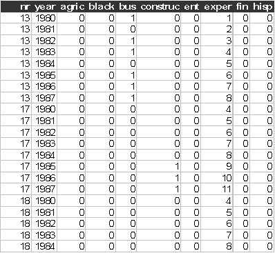
The first few rows and columns of the data for the univariate models look like:

Start Sabre and specify transcript file:
out union-wage.log
data nr year agric black bus construc ent exper fin hisp poorhlth hours &
manuf married min nrthcen nrtheast occ1 occ2 occ3 occ4 occ5 occ6 occ7 &
occ8 occ9 per pro pub rur south educ tra trad union lwage d81 d82 d83 &
d84 d85 d86 d87 expersq
read wagepan.dat
Suggested exercise
Wage equation
(1) Estimate a linear model for lwage (log of hourly wage) with the covariates (educ, black, hisp, exper, expersq, married, union, d8m, m=1,2,…,7) and the respondent identifier (nr) random effect. Is this random effect significant? Use 64 quadrature points to estimate this model?
Trade Union membership
(2) Estimate a logit model for trade union membership (union), with the covariates. (black, hisp, exper, educ, poorhlth, married, rur,nrthcen, nrtheast, south and allow for the respondent identifier (nr) random effect. Is this random effect significant? How many quadrature points should we use to estimate this model?
Joint Model
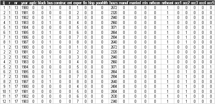
We have stacked the data for this part (union-wage.dat), the first few columns and rows look like

To read this data you need:
out union-wage.log
data ij r nr year agric black bus construc ent exper fin hisp poorhlth &
hours manuf married min nrthcen nrtheast occ1 occ2 occ3 occ4 occ5 &
occ6 occ7 occ8 occ9 per pro pub rur south educ tra trad union y d81 &
d82 d83 d84 d85 d86 d87 expersq r1 r2
read union-wage.dat
(3) Using the model specifications for log(wages) and trade union membership you have just used, estimate a joint model of the determinants of log(wages) and trade union membership. What is the magnitude and significance of the correlation between the random effects for log(wages) and union membership? How does the magnitude and significance of the direct effect of union in the wage equation change? What are the reasons for this? Have any other features of the models changed? What does this imply?
Below are the commands we used
case nr
yvar y
model b
rvar r
family second=g
constant first=r1 second=r2
trans r1_black r1 * black
trans r1_hisp r1 * hisp
trans r1_exper r1 * exper
trans r1_educ r1 * educ
trans r1_poorhlth r1 * poorhlth
trans r1_married r1 * married
trans r1_rur r1 * rur
trans r1_nrthcen r1 * nrthcen
trans r1_nrtheast r1 * nrtheast
trans r1_south r1 * south
trans r2_educ r2 * educ
trans r2_black r2 * black
trans r2_hisp r2 * hisp
trans r2_exper r2 * exper
trans r2_expersq r2 * expersq
trans r2_married r2 * married
trans r2_union r2 * union
trans r2_d81 r2 * d81
trans r2_d82 r2 * d82
trans r2_d83 r2 * d83
trans r2_d84 r2 * d84
trans r2_d85 r2 * d85
trans r2_d86 r2 * d86
trans r2_d87 r2 * d87
nvar 11
mass second=64
fit r1_black r1_hisp r1_exper r1_educ r1_poorhlth r1_married r1_rur &
r1_nrthcen r1_nrtheast r1_south r1 &
r2_educ r2_black r2_hisp r2_exper r2_expersq r2_married r2_union &
r2_d81 r2_d82 r2_d83 r2_d84 r2_d85 r2_d86 r2_d87 r2
dis m
dis e
stop
References
Rabe-Hesketh, S., and Skrondal, A., (2005), Multilevel and Longitudinal Modelling using Stata, Stata Press, Stata Corp, College Station, Texas
Vella, F., and Verbeek, M., (1998), Whose wages do unions raise? A dynamic model of unionism and wage rate determination for young men. Journal of Applied Econometrics, 13, 163-183.
Wooldridge, J, M., (2002), Econometric Analysis of Cross
Section and Panel Data, MIT Press,