Exercise L5, ordered
response
Wiggins et al (1991) studied attitudes to abortion using a
subset of the data from the British Social Attitudes (BSA) Survey. The BSA
Survey is a multistage clustered random sample of adults (aged 18 and over)
living in private households in
A subset of individuals, from the 1983 BSA survey, were followed each year until 1986. The subset of the data we use here was used by Rabe-Hesketh and Skrondal (2005, exercise 5.5) for modelling the ordinal response strength of support for legalising abortion. The data are limited to the respondents who provided valid values for all 4 years of follow up. The strength of support each year was judged by combining the responses (yes/no) on 7 different circumstances in which abortion should be legal. The questions relate to circumstances such as “The woman became pregnant as a result of rape”, and “The woman decides on her own that she does not wish to have a child”. Differences in magnitude of circumstances outside the woman’s control are ignored and the respondent’s total score is obtained by adding up the responses on the 7 different questions.
Data description
Number of observations (rows): 1056
Number of variables (columns): 16
Variables:
district=district identifier
person=respondent/individual identifier
year=year (1,2,3,4)
score=the number of questions (circumstances) to which the respondent answered yes
age=respondent’s age in years
male=1 if respondent is male, 0
otherwise
nscore =1 if score=0,1,2 (as the values 0,1,2 for score are rare)
nscore =2 if score =3
nscore =3 if score =4
nscore =4 if score =5
nscore =5 ff score =6
dr2 = if the respondent’s religion is protestant (catholic is the reference category)
dr3 = if the respondent’s religion is other religion
dr4 = if the respondent’s religion is agnostic
dp2 = if the respondent votes labour (conservative is the reference category)
dp3 = if the respondent votes liberal
dp4 = if the respondent votes other
dp5 = if the respondent votes none
dc2 = if the respondent’s self assessed social class is middle (upper is the reference category)
dc3 = if the respondent’s self assessed social class is lower
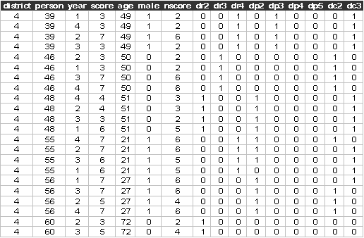
The first few lines of abortion2.dat look like:

Start Sabre and specify transcript file:
out abortion.log
data district person year score
age male nscore dr2 dr3 dr4 dp2 dp3 dp4 &
dp5 dc2 dc3
read abortion2.dat
Suggested exercise
(1) Estimate an ordered logit model to nscore, without covariates
(2) Allow for the person identifier (person) random effect, is this random effect significant? How many quadrature points should we use to estimate this model?
(3) Add the explanatory variables male age and the three sets of dummy variables created in part (2) above . How does the magnitude of the person random effect change? Are any of these individual characteristics significant in this model? Do the results make intuitive sense?
(4) Repeat parts (1), (2) using district as the random effect, to do this you will need to use a version of the data set sorted by district, this is called abortion3.dat, i.e.
data district person year score
age male nscore dr2 dr3 dr4 dp2 dp3 dp4 &
dp5 dc2 dc3
read abortion3.dat
case district
Does the significance of the explanatory variables change? Do the results make intuitive sense?
(5) Interpret your preferred model. Can your preferred model be simplified?
(6) Are there any interaction effects you would like to try to add to this model? Why?
Sabre does not yet allow for the nesting of respondents within districts and respondents over different years.
References
Rabe-Hesketh, S., and Skrondal, A., (2005), Multilevel and Longitudinal Modelling using Stata, Stata Press, Stata Corp, College Station, Texas
Wiggins, R. D., Ashworh, K., O’Muircheartaigh, C. A., Galbraith, J. J., (1991), Multilevel analysis of attitudes to abortion, Journal of the Royal Statistical Society, Series D, 40, 225-234.