Exercise L6, ordered response
Koch et al (1989) analysed the clinical trial data from 2 centres that compared two groups for respiratory illness. Eligible patients were randomised to treatment or placebo groups at each centre. The respiratory status (ordered response) of each patient prior to randomisation and at 4 later visits to the clinic was determined.
The number of young patients in the sample is 110. The version of the data set (respiratory2.dat) we use was also used by Rabe-Hesketh and Skrondal (2005, exercise 5.1).
Data description
Number of observations (rows): 555
Number of variables (columns): 21
Variables:
center=Centre (1,2)
drug=1 if patient was allocated to the treatment group, 0 if placebo
male=1 if patient was male, 0 otherwise
age=patient’s age
bl= patient’s respiratory status prior to randomisation
v1= patient’s respiratory status at visit 1 (0: terrible; 1: poor; 2: fair; 3: good; 4: excellent)
v2= patient’s respiratory status at visit 2 (0: terrible; 1: poor; 2: fair; 3: good; 4: excellent)
v3= patient’s respiratory status at visit 3 (0: terrible; 1: poor; 2: fair; 3: good; 4: excellent)
v4= patient’s respiratory status at visit 4 (0: terrible; 1: poor; 2: fair; 3: good; 4: excellent)
patient=Patient identifier (1,2,…,110)
status = the stacked versions of bl and vt, with 1 added to each
value
r1 = 1 if this is the response for bl (pre randomisation), 0 otherwiser2 = 1 if this is the response for visit 1, 0 otherwiser3 = 1 if this is the response for visit 2, 0 otherwiser4 = 1 if this is the response for visit 3, 0 otherwiser5 = 1 if this is the response for visit 4, 0 otherwisebld = 1 if this is the pre randomisation response, 0 otherwise
trend = 0 or visit (1,2,3,4)
base = 1 for all post treatment data, 0 for pre treatment data
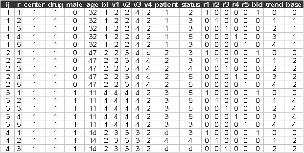
The data are sorted by patient within center. The first few lines of respiratory2.dat look like:

Start Sabre and specify transcript file:
out respiratory.log
data ij
r center drug male age bl
v1 v2 v3 v4 patient status r1 r2 r3 r4 &
r5 bld trend base
read respiratory2.dat
Suggested exercise:
(1) Estimate an ordered logit model for status without any covariates.
(2) Estimate the ordered logit model for status, allowing for the patient random effect. Are the random patient effects significant? How many quadrature points should we use to estimate this model?
(3) Re-estimate the model allowing for drug, male, age and base. How does the magnitude of the patient random effect change? Are any of these explanatory variables significant in this model? Do the results make intuitive sense?
(4) Calculate an interaction between trend and drug, add the linear trend variable to the model, then add the interaction between trend and drug. Does the impact of treatment vary with visit?
(5) Repeat parts (1) and (2) using center for the random effect for status, to do this you will need to use a version of the data set sorted by center, this is called respiratory3.dat. i.e.
data ij
r center drug male age bl
v1 v2 v3 v4 patient status r1 r2 r3 r4 &
r5 bld trend base
read respiratory3.dat
Does the significance of the explanatory variables change? Do the results make intuitive sense?
(6) Interpret your preferred model, can your preferred model be simplified?
(7) Are there any interaction effects you would like to try to add to this model? Why?
Sabre does not yet allow for the nesting of patients within centres and patients over visits.
References
Koch, G. G., Car, G. J., Amara,
A., Stokes, M. E., and Uryniak, T. J., (1989),
Categorical data analysis. In
Rabe-Hesketh, S., and Skrondal, A., (2005), Multilevel and Longitudinal Modelling using Stata, Stata Press, Stata Corp, College Station, Texas