Exercise L7, duration data

In 1986, the ESRC funded the Social Change and Economic Life Initiative (SCELI). Under this initiative work and life histories were collected for a sample of individuals from 6 different geographical areas in the UK. One of these locations was Rochdale. The data set (roch2.dat) contains annual data on male respondents’ residential behaviour since entering the labour market. These are residence histories on 348 Rochdale men aged 20 to 60 at the time of the survey. We are going to use these data in the study of the determinants of residential mobility.

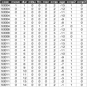
Data description

Number of observations (rows): 6349

Number of variables (columns): 10

Variables:

case= respondent number

move= residential move (0=no; 1=yes)

dur=number of years since last move

mbu= marriage break-up during the year (0=no; 1=yes)

fm= first marriage during the year (0=no; 1=yes)

mar= married at the beginning of the year (0=no; 1=yes)

emp= employment at the beginning of the year (1=self employed; 2=employee; 3=not working)

age= (age-30) years

emp2=1 if employment at the beginning of the year is employee; 0 otherwise

emp3=1 if employment at the beginning of the year is not working; 0 otherwise

Note that the variable dur, which measures the number of years since the last move is endogenous, i.e. it is internally related to the process of interest.

The first few lines of roch2.dat look like

Start Sabre and specify transcript file:

out roch.log

data case move dur mbu fm mar emp age emp2 emp3

read roch2.dat

Suggested Exercise

(1) Create quadratic (age2) and cubic (age3) terms in age to allow more flexibility in modelling this variable (i.e. to allow for a non-linear relationship).

(2) Specify the binary response variable (move) and fit a cloglog model to the explanatory variables age dur fm mbu mar emp2 emp3. Add the age2 and age3 effects to this mode, are they significant. What does this tell you about residential mobility.

(3) Add the case random effect to the model estimated in part 2, is it significant? How many quadrature points should we use to estimate this model? Interpret you results. Can the model be simplified?

How do things change between the independent and random effect model?