Sabre

 

Multilevel Multiprocess Modelling Examples

 

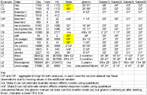
The results of the comparison between Stata, gllamm and Sabre (#processors) in terms of CPU time in hours, minutes(‘) and seconds (“) on 15 example data sets (C=cross sectional, L=longitudinal) are listed in the table below. Many of the published data sets in this table are quite small and as such are not very computationally demanding for Sabre. All the examples, exercises, data sets, training materials and software may be downloaded from this site .

 

 

All the computations reported above were performed on Lancaster University's High Performance Computing facility, which consists of an array of 103 dual-processor Sun-Blade workstations, each having between 1 and 8 gigabytes of memory. They are connected to a fileserver with 1300 gigabytes of disk storage. Sixteen of the workstations have "Myrinet" cards installed to allow very high speed communication between them, supporting parallel programs which distribute large amounts of data. The non-Myrinet connections run at 100 Mbits.  Jobs are submitted to the array from the HPC front-end machine through the Sun Grid Engine/Codine queuing system hosted on the file server. This in turn distributes each submitted job to one of the many execution hosts, or holds it until a host becomes available. Users may submit large numbers of individual batch jobs, interactive jobs, or parallel, or message passing programs using either MPI or PVM. In all of the computational comparisons we used workstations without the Myrinet cards. The Sun Blade workstations are 64 bit with 1 GB+ of RAM, they run at 0.9 GHz. The HPC compiler is Sun Fortran 95 8.1We also ran many of the single processor examples on a Celeron 2.8 GHz, 256 MB of RAM, Windows XP. In this case Sabre was compiled using the Intel Fortran 9.0 Compiler. The Celeron generally finishes in ½ the time it takes the HPC processors. The HPC is now 3 years old, and is due to be replaced in April 06. However, it is the relative timings that are important in the Table.

 

The shaded elements of the Stata column are for the linear model using the Stata command xtreg, to estimate a random effects linear model using MLE. The integrated likelihood for the normal distributed random effects, normal linear model has a closed form. There are currently no Stata commands for bivariate random effect models, so no comparison with Stata is possible, hence the cells with ‘not applicable’ (n/a) in them. The gllamm timings with a plus sign are from an estimated lower limit (based on jobs run on a subset of the data), or from the point where we decided that we could not wait any longer for gllamm to end on its own.

 

The non-shaded results we quote are for standard quadrature in gllamm. The same number of quadrature points are used in the Stata, gllamm and Sabre comparisons. The number of quadrature points varies by example, depending on the number needed to give a good approximation to the likelihood. We have not used the gllamm adaptive quadrature algorithm in these comparisons. The argument for using adaptive quadrature arises from the fact that Gaussian quadrature can perform badly when there are insufficient locations under the peak of the integrated likelihood. Adaptive quadrature is used to shift the quadrature points in order to improve the adequacy of the approximation. Adaptive quadrature generally requires fewer quadrature points than standard quadrature to provide the same approximation of the likelihood. However, there is very little computational burden in Sabre to increasing the number of quadrature points.

 

The timings for examples C3 and C4 are the joint timings for two sets of estimates. In both C3 and C4 the second data set has one more explanatory variable and fewer cases. The analysis with the addition variable has some missing values. In both the C3 and C4 data sets, observations with missing values were deleted.

 

Sabre (1) clearly outperforms gllamm on all the data sets. Stata only outperforms Sabre (1) when it uses the MLE procedure (C1, C2, L1, L2, L3).

 

Why is Stata slower than Sabre? This is because Stata is distributed in a compiled version that will run on a range of different processors. Stata do not distribute a different compiled version for every processor, and there is typically just one version for each operating system. Why is gllamm slower than Stata? This is because gllamm is an add-on, written in an interpreted language, i.e. the statements are translated to machine code as they run, which happens every time a loop is executed. The same algorithm in a compiled language (and optimised by the compiler to take advantage of the host processor) will run many times faster. There also algorithmic differences too, e.g. Sabre's analytical rather than numeric calculation of the derivatives.

 

If seconds matter, there can be some saving by going parallel on small data sets. However, looking down the table we see that the first real advantage of using Sabre first appears in example C6 (visit-prescribe), which involved the estimation of a bivariate Poisson model. Gllamm takes nearly 2 days while Sabre (1) only takes 2’ 21” which goes down to 20” with 8 processors. Sabre (1) is nearly 3000 times faster than gllamm in estimating this model..

 

The crucial illustration occurs with respect to examples L7 and L8. These examples are from a study that provides the first estimates of the determinants of employer search in the UK using duration modelling techniques. It involves modelling a job vacancy duration until either it is successfully filled or withdrawn from the market. For further detail see the online paper.

 

In example L7 we treat the 'filled' and 'lapsed' datasets as if they were independent, both data sets have 390,432 binary observations (at the weekly level) on 12,840 vacancies. For the first risk ('filled') the final response for each vacancy is 1 at the point where the vacancy fills, and similarly for the ('lapsed') risk. At all other weeks the responses are zero. There are 7,234 filled vacancies and 5,606 lapsed vacancies.

 

The separate 'filled' and 'lapsed' duration models can be fitted in Stata using xtclog, gllamm and Sabre. For each type of risk we used a 26-piece non-parametric baseline hazard with 55 covariates and 12-point Gaussian quadrature. Stata took just under 3 days to estimate each model. After 3 months gllamm had still failed to converge.

 

The combined dataset, (example L8) has 780,864 observations, each of the 12,840 vacancies being represented twice, with each sequence of vacancy responses ending in a 1 at the point where the vacancy is filled for a 'filled' risk, the 'lapsed' risk is right censored at this point and vice versa for a 'lapsed' risk. Sabre 4.0 and gllamm can estimate a model which allows for a correlation between the risks, this option is currently not available in Stata. Sabre (1) takes about 2.5 days to estimate the correlated risks model, by going parallel on 8 processors this time can be cut down to ½ a day. We estimate that gllamm will take over 3 years on our HPC.